Example usage

Here we will demonstrate how to use SeisScan to detect and locate earthquakes.

We will first read data from IRIS full wavefield experiment.

We will then proceed to compute characteristic function and backproject them for detection and location.

import warnings
warnings.filterwarnings('ignore')

import os
import sys
import glob
from obspy import UTCDateTime, Stream
from obspy.geodetics import gps2dist_azimuth
from matplotlib import pyplot as plt
from cartopy import crs as ccrs
from dask.distributed import Client as dask_Client

import seisscan as ss
print(ss.__version__)

0.1.0

Start DASK for parallel processing

n_workers = os.cpu_count() - 2
dask_client = dask_Client(n_workers=n_workers)

Read example data

event_dict, st, inventory, subnetworks, model_name = ss.read_example()

Let’s extract event information

evt0 = UTCDateTime(event_dict["evt0"])    # event origin time
evlo = event_dict["evlo"]                 # event longitude
evla = event_dict["evla"]                 # event latitude
evdp = event_dict["evdp"]                 # event depth (km)
mag = event_dict["mag"]                   # event magnitude

Print the Subnetworks

subnetworks

[{'reference': '1002', 'secondaries': ['1001', '1003']},
 {'reference': '1041', 'secondaries': ['5019', '5020', '5025', '5026']},
 {'reference': '1073', 'secondaries': ['5004', '5005', '5012', '5013']},
 {'reference': '1128', 'secondaries': ['1127', '1129']},
 {'reference': '2005', 'secondaries': ['2004', '2006']},
 {'reference': '2048', 'secondaries': ['2047', '2049']},
 {'reference': '3002', 'secondaries': ['3001', '3003']},
 {'reference': '3048', 'secondaries': ['3047', '3049']}]

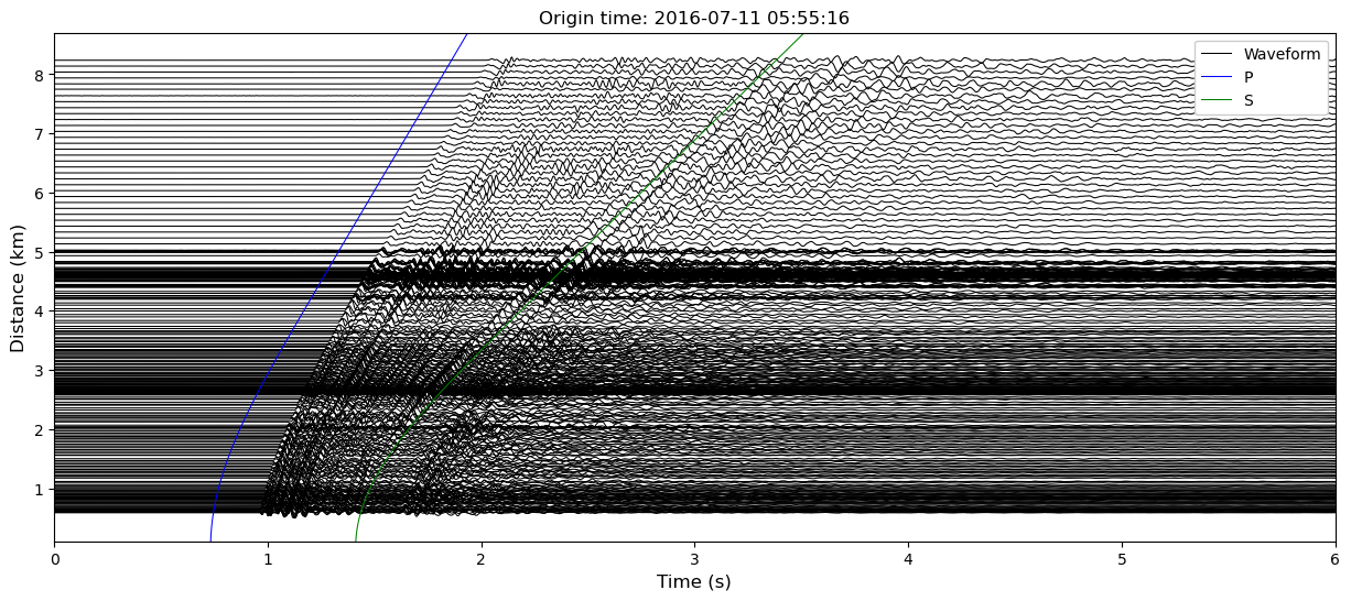
Plot a record section of the stream

channel = "DPZ"

fig = ss.prs(st.select(channel=channel),
             evt0, evlo, evla, evdp, scale=0.1, model_name=model_name,
             xmin=0.0, xmax=6.0, width=15, height=6, handle=True)

Select Stream for the stations in the Subnetworks

st_sel = Stream()

for subnetwork in subnetworks:
    reference = subnetwork["reference"]
    secondaries = subnetwork["secondaries"]

    st_sel += st.select(station=reference)

    for secondary in secondaries:
        st_sel += st.select(station=secondary)

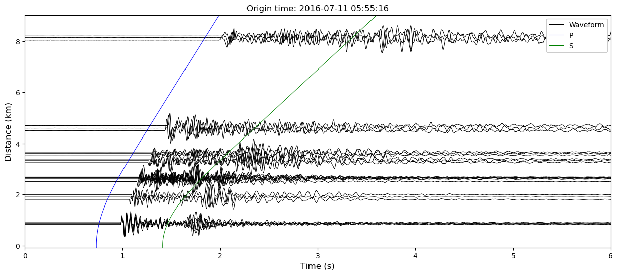
Plot a record section of the selected stream

channel = "DPZ"

fig = ss.prs(st_sel.select(channel=channel),
             evt0, evlo, evla, evdp, scale=0.5, model_name=model_name,
             xmin=0.0, xmax=6.0, width=15, height=6, handle=True)

Pre-process the selected stream

#--- take a copy of the selected stream
st_proc = st_sel.copy()

#--- detrend the data
st_proc.detrend(type='linear');

#--- remove instrument response
pre_filt = [0.1, 0.2, 200.0, 250.0]   # Hz
st_proc.remove_response(output='VEL', pre_filt=pre_filt);

#--- rotation from 'Z12' to 'ZNE
st_proc.rotate('->ZNE', inventory=inventory);

#--- filter
f1, f2 = 25.0, 75.0
st_proc.select(component='Z').filter('bandpass', freqmin=f1, freqmax=f2);

f1, f2 = 10.0, 30.0
st_proc.select(component='N').filter('bandpass', freqmin=f1, freqmax=f2);
st_proc.select(component='E').filter('bandpass', freqmin=f1, freqmax=f2);

#--- Merge traces with similar seed_id
st_proc.merge(method=1, fill_value=0);

#--- Trim the stream so that every trace has similar starttime and endtime
starttime = min([tr.stats.starttime for tr in st_proc])
endtime = max([tr.stats.endtime for tr in st_proc])
st_proc.trim(starttime, endtime, pad=True, fill_value=0);

Compute characteristic function (Local Similarity)

channels = ['DPZ', 'DPN', 'DPE']
w = 0.75 # window length in seconds
dt = 0.05 # stride in seconds
max_lag = 0.1 # maximum lag in seconds

st_r = Stream()
st_dls = Stream()

for channel in channels:
    _, _, _, _, _, st_dls_ = ss.do_ls(st_proc, channel, subnetworks=subnetworks, w=w, dt=dt, max_lag=max_lag, dask_client=dask_client)
    st_dls += st_dls_

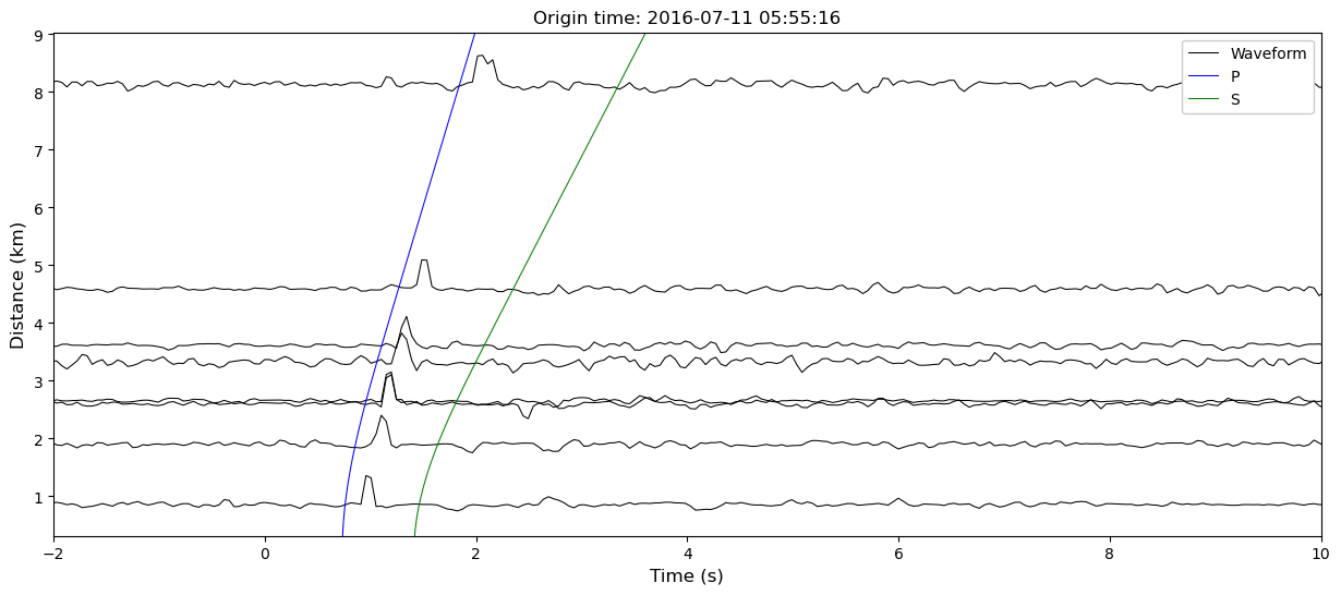
Plot a record section of the characteristic functions

channel = "DPZ"

fig = ss.prs(st_dls.select(channel=channel),
             evt0, evlo, evla, evdp, scale=0.5, model_name=model_name,
             xmin=-2, xmax=10, width=15, height=6, handle=True)

Prepare a travel time lookup table for P- and S-wave

#--- parameters for travel time calculation
min_dist_k, max_dist_k, step_dist_k = 0.0, 50.0, 2.0    # start, end and step for epicentral distance in km
min_dep_k, max_dep_k, step_dep_k = 0.0, 15.0, 0.5       # start, end and step for depth in km

#--- perform calculation for P-wave
phase = 'p'
mod_dist_r1, mod_dep_r1, mod_ttp_r2, computation_time = ss.prepare_traveltime_lookup_table(
    min_dist_k, max_dist_k, step_dist_k,
    min_dep_k, max_dep_k, step_dep_k,
    phase, model_name=model_name, dask_client=dask_client
)

#--- perform calculation for S-wave
phase = 's'
_, _, mod_tts_r2, computation_time = ss.prepare_traveltime_lookup_table(
    min_dist_k, max_dist_k, step_dist_k,
    min_dep_k, max_dep_k, step_dep_k,
    phase, model_name=model_name, dask_client=dask_client
)

Backprojection

Define parameters for backprojection

#--- prepare source grid
min_lon, max_lon = -97.75, -97.59        # deg
min_lat, max_lat = 36.59, 36.64          # deg
min_dep, max_dep = 0, 15                 # km
step_x, step_y, step_z = 0.25, 0.25, 0.25  # km

#--- calculation of time window
w = 0.25 # window size in seconds
o = 0.80 # overlap fraction for successive window

#--- Positioon of the brightness value on the time window: 'start', 'mid' or 'end'
pos = 'mid'

#--- components for calculation
p_components = ['Z']
s_components = ['N', 'E']

Compute 4-D (time-space) brightness function

brightness4 = ss.do_bp(st_dls, dask_client, w,
            min_lon, max_lon, min_lat, max_lat, min_dep, max_dep, step_x, step_y, step_z,
            mod_dist_r1, mod_dep_r1, mod_ttp_r2, mod_tts_r2,
            o=o,
            pos=pos,
            p_components=p_components,
            s_components=s_components)

Get backprojected solution

evt0_bp, evlo_bp, evla_bp, evdp_bp = brightness4.get_solution()

print(f'Backprojected event origin time: {evt0_bp.strftime("%Y-%m-%d %H:%M:%S.%f")}')
print(f'Backprojected event longitude: {evlo_bp:0.04f} deg.')
print(f'Backprojected event latitude: {evla_bp:0.04f} deg.')
print(f'Backprojected event depth: {evdp_bp:0.02f} km.')

Backprojected event origin time: 2016-07-11 05:55:16.578000
Backprojected event longitude: -97.6913 deg.
Backprojected event latitude: 36.6170 deg.
Backprojected event depth: 2.75 km.

Difference between the backprojected and analyst solution

# Difference between backprojected and analyst origin time
evt0_diff = evt0_bp - evt0

# Distance between backprojected and analyst epicenter
dist_meter, _, _ = gps2dist_azimuth(evla, evlo, evla_bp, evlo_bp)
dist_km = dist_meter / 1000

# Difference between backprojected and analyst depth
depth_diff = evdp_bp - evdp

print(f'Difference between backprojected and analyst origin time: {evt0_diff:0.02f} seconds.')
print(f'Distance between backprojected and analyst epicenter: {dist_km:0.02f} km.')
print(f'Difference between backprojected and analyst depth: {depth_diff:0.02f} km.')

Difference between backprojected and analyst origin time: 0.19 seconds.
Distance between backprojected and analyst epicenter: 0.22 km.
Difference between backprojected and analyst depth: -0.25 km.

Plot the results

Get reference station coordinates

station_list = sorted(list(set([tr.stats.station for tr in st_dls])))
stlo_list = [st_dls.select(station=station)[0].stats.sac.stlo for station in station_list]
stla_list = [st_dls.select(station=station)[0].stats.sac.stla for station in station_list]

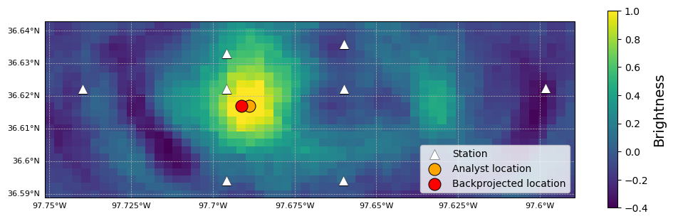
Plot XY brightness slices at the backprojected source

fig = plt.figure(figsize=(12,12))
projection = ccrs.PlateCarree()
ax = fig.add_subplot(projection=projection)

# axes gridlines and ticklabels
gl = ax.gridlines(ls='--', lw=0.5)
gl.bottom_labels = True
gl.left_labels = True
gl.xlabel_style = {'fontsize':8}
gl.ylabel_style = {'fontsize':8}

# Plot brightness
s = brightness4.plot_slice(ax, plane='xy', t=evt0_bp)
s.set_clim(vmin=-0.4, vmax=1.0)

cbar = fig.colorbar(s, shrink=0.3);
cbar.ax.tick_params(labelsize=10)
cbar.ax.set_ylabel('Brightness', fontsize=14)

# plot stations
ax.scatter(stlo_list, stla_list, marker='^', ec='k', fc='w', lw=0.25, s=100, label='Station')

# plot analyst event
ax.scatter(evlo, evla, marker='o', ec='k', fc='orange', lw=0.75, s=150, label='Analyst location')

# plot backprojected event
ax.scatter(evlo_bp, evla_bp, marker='o', ec='k', fc='red', lw=0.75, s=150, label='Backprojected location')

#--- legend
ax.legend(loc=4);

# fig.savefig(f'brightness_XY_slice.png', bbox_inches="tight")

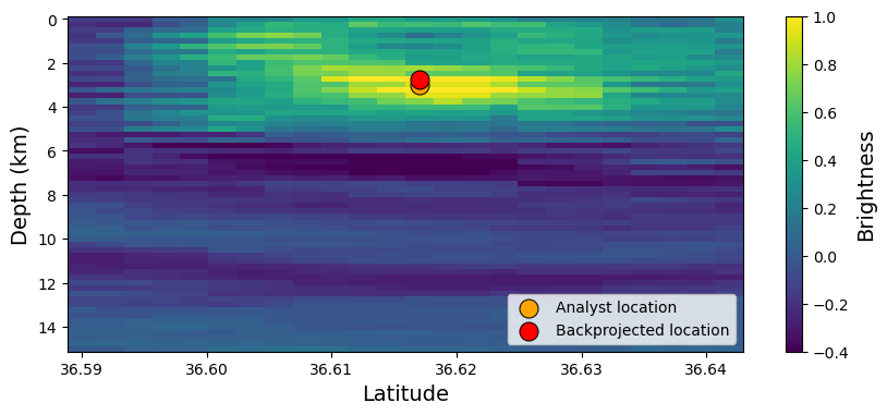
Plot YZ brightness slices at the backprojected source

fig = plt.figure(figsize=(10,4))
ax = fig.add_subplot(1,1,1)
ax.invert_yaxis()

ax.set_xlabel('Latitude', fontsize=14)
ax.set_ylabel('Depth (km)', fontsize=14);

#--- Plot brightness
s = brightness4.plot_slice(ax, plane='yz', t=evt0_bp)
s.set_clim(vmin=-0.4, vmax=1.0)

cbar = fig.colorbar(s, shrink=1.0);
cbar.ax.tick_params(labelsize=10)
cbar.ax.set_ylabel('Brightness', fontsize=14)

#--- plot analyst event
ax.scatter(evla, evdp, marker='o', ec='k', fc='orange', lw=0.75, s=150, label='Analyst location')

#--- plot backprojected event
ax.scatter(evla_bp, evdp_bp, marker='o', ec='k', fc='red', lw=0.75, s=150, label='Backprojected location')

#--- legend
ax.legend(loc=4);

# fig.savefig(f'brightness_YZ_slice.png', bbox_inches="tight")

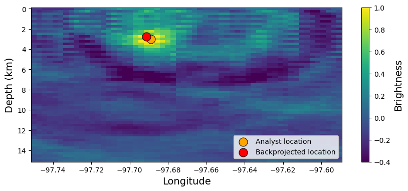
Plot ZX brightness slices at the backprojected source

fig = plt.figure(figsize=(10,4))
ax = fig.add_subplot(1,1,1)
ax.invert_yaxis()

ax.set_xlabel('Longitude', fontsize=14)
ax.set_ylabel('Depth (km)', fontsize=14);

#--- Plot brightness
s = brightness4.plot_slice(ax, plane='zx', t=evt0_bp)
s.set_clim(vmin=-0.4, vmax=1.0)

cbar = fig.colorbar(s, shrink=1.0);
cbar.ax.tick_params(labelsize=10)
cbar.ax.set_ylabel('Brightness', fontsize=14)

# #--- plot analyst event
ax.scatter(evlo, evdp, marker='o', ec='k', fc='orange', lw=0.75, s=150, label='Analyst location')

# #--- plot backprojected event
ax.scatter(evlo_bp, evdp_bp, marker='o', ec='k', fc='red', lw=0.75, s=150, label='Backprojected location')

# #--- legend
ax.legend(loc=4);

# fig.savefig(f'brightness_ZX_slice.png', bbox_inches="tight")

get the backprojected stack

brightness_stack = brightness4.get_stack()
times = brightness_stack.get_times(reftime=evt0_bp)      # time of the stack
b_r1 = brightness_stack.b_r1                             # brightness of the stack

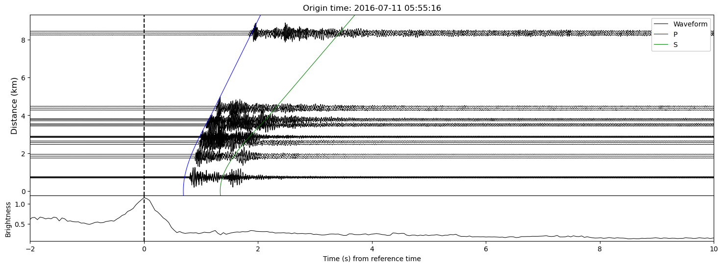
Plot the backprojected stack along with record section of the master station waveforms

#--- Channel codes for this example are DPZ, DPN, DPE
channel = 'DPZ'

#--- create figure and axes
fig = plt.figure(figsize=(18,6))
gs = fig.add_gridspec(5, hspace=0.0)
ax = fig.add_subplot(gs[0:4,0])
ax2 = fig.add_subplot(gs[4,0], sharex=ax)

ax2.set_ylabel('Brightness')
ax2.set_xlabel('Time (s) from reference time')

#--- remove xticklabels from ax
[label.set_visible(False) for label in ax.get_xticklabels()]

#--- plot record section of the reference waveforms
ss.prs(st_proc.select(channel=channel), evt0_bp, evlo_bp, evla_bp, evdp_bp, ax=ax, model_name=model_name, xmin=-2, xmax=10)
ax.axvline(0, color='k', ls='--')

# #--- plot stack
ax2.plot(times, b_r1, color='k', lw=0.75)
ax2.axvline(0, color='k', ls='--');

# fig.savefig(f'lsbp_stack_{channel}.png')

Close DASK client

dask_client.close()