Data Structure

The following datasets are required:

1. Obspy.Stream with station metadata added.

2. Station Subnetworks.

Imports

from obspy import UTCDateTime
from obspy.core import AttribDict
from obspy.clients.fdsn import Client
client = Client("IRIS")

import seisscan as ss

ObsPy.Stream with station metadata added

An ObsPy.Stream object contains a number of Obspy.Trace objects. Station coordinates are to be attached to each Obspy.Trace. Optionally, station response information can also be attached to Obspy.Trace. Let’s follow the ObsPy example to download data and metadata.

# Define starttime and endtime
starttime = UTCDateTime("2010-02-27T06:45:00.000")
endtime = starttime + 60

# Download Stream
st = client.get_waveforms("IU", "ANMO", "00", "LHZ", starttime, endtime, attach_response=True)

#- Download station metadata
inventory = client.get_stations(network="IU", station="ANMO", location="00", channel="LHZ",
                                starttime=starttime, endtime=endtime, level="response")

Station coordinates can be attached to each Obspy.Trace as shown below.

# loop over st
for tr in st:
    coordinates = inventory.get_coordinates(tr.id, datetime=tr.stats.starttime)
    tr.stats.sac = AttribDict()
    tr.stats.sac.stlo = coordinates['longitude']
    tr.stats.sac.stla = coordinates['latitude']
    tr.stats.sac.stel = coordinates['elevation']

# print stats of the first
print(st[0].stats)

               network: IU
               station: ANMO
              location: 00
               channel: LHZ
             starttime: 2010-02-27T06:45:00.069538Z
               endtime: 2010-02-27T06:45:59.069538Z
         sampling_rate: 1.0
                 delta: 1.0
                  npts: 60
                 calib: 1.0
_fdsnws_dataselect_url: http://service.iris.edu/fdsnws/dataselect/1/query
               _format: MSEED
                 mseed: AttribDict({'dataquality': 'M', 'number_of_records': 1, 'encoding': 'STEIM2', 'byteorder': '>', 'record_length': 512, 'filesize': 512})
            processing: ['ObsPy 1.4.0: trim(endtime=UTCDateTime(2010, 2, 27, 6, 46, 0, 69538)::fill_value=None::nearest_sample=True::pad=False::starttime=UTCDateTime(2010, 2, 27, 6, 45, 0, 69538))']
              response: Channel Response
        From m/s (Velocity in Meters Per Second) to counts (Digital Counts)
        Overall Sensitivity: 3.25959e+09 defined at 0.020 Hz
        3 stages:
                Stage 1: PolesZerosResponseStage from m/s to V, gain: 1952.1
                Stage 2: CoefficientsTypeResponseStage from V to counts, gain: 1.67772e+06
                Stage 3: CoefficientsTypeResponseStage from counts to counts, gain: 1
                   sac: AttribDict({'stlo': -106.457133, 'stla': 34.945981, 'stel': 1671.0})

Alternate method to attach station metadata

Alternatively, the function SeisScan.read_fdsn can be used to retrive ObsPy.Stream with station metadata attached. It utilizes FDSN web service client for ObsPy to request ObsPy.Stream object and station metadata (station coordinates and response information). Finally, it attaches the metadata information to each ObsPy.Trace of the Obspy.Stream object and returns the Obspy.Stream object. The following example is similar to the previous example.

starttime = UTCDateTime("2010-02-27T06:45:00.000")
endtime = starttime + 60

st = ss.read_fdsn(starttime, endtime, "IU", "ANMO", "00", "LHZ", provider="IRIS")

Station Subnetworks

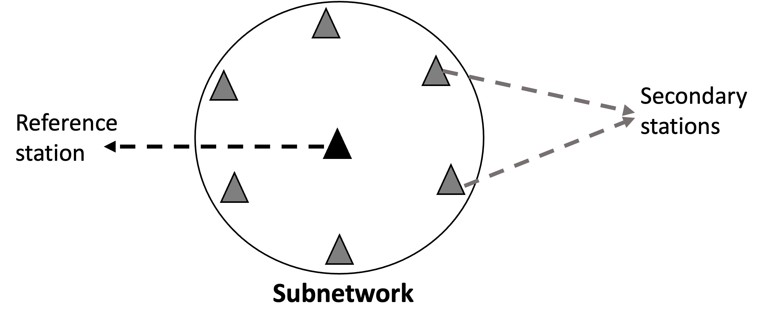
A Subnetwork is a station cluster where the central station is defined as the reference station, whereas the remaining stations are called secondary stations. It is represented by a dictionary with two keys, reference and secondaries. The value of reference is the central station code and the value of secondaries is a list of secondary station codes. An example is given below.

subnetwork = {"reference": "STA01", "secondaries":["STA02", "STA03"]}

A Subnetworks is a list of Subnetwork. For example,

subnetwork_1 = {"reference": "STA01", "secondaries":["STA02", "STA03"]}
subnetwork_2 = {"reference": "STA11", "secondaries":["STA12", "STA13"]}
subnetwork_3 = {"reference": "STA21", "secondaries":["STA22", "STA23"]}
subnetworks = [subnetwork_1, subnetwork_2, subnetwork_3]

import os
os.path.exists("seisscan_images/subnetwork.jpg")

True